Decision Trees: Why Nested Rules Still Matter in the LLM Era

A recent top Hacker News post resurfaced Amazon's MLU Explain visual guide on decision trees, reminding many practitioners that some of the most useful ML tools are also the simplest. Decision trees are nothing more than nested if/else rules, yet they can model surprisingly complex patterns while remaining fully inspectable.

Core Concepts

Decision Tree Fundamentals

A decision tree makes predictions by walking down a sequence of yes/no tests on input features:

1. Start at the root node.
2. Test a feature against a threshold (e.g., age <= 35?).
3. Follow the branch (yes/no) to the next node.
4. Repeat until reaching a leaf node, which outputs a prediction.

This framework supports:

• Classification: leaves output class labels or class probabilities.
• Regression: leaves output continuous values (e.g., an average target value).

Because each prediction corresponds to a concrete path of rules, trees are inherently interpretable.

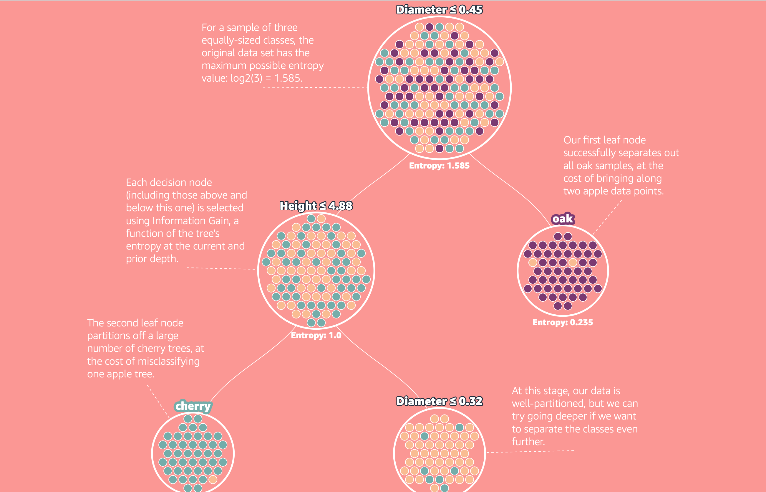
Entropy and Information Gain

To build a tree from data, we need a way to decide which feature and threshold to split on at each node.

• Entropy measures label disorder in a node:

$$H = - \sumi pi \log2 pi$$

where (p_i) is the proportion of samples in class (i).

• Information gain measures how much entropy decreases after a split:

$$\text{Gain} = H(\text{parent}) - \sum{k} \frac{nk}{n} H(\text{child}_k)$$

We evaluate candidate splits and choose the one with the highest information gain.

The ID3 Algorithm

The classic ID3 algorithm builds a tree recursively:

1. Compute the entropy of the current node.
2. For each feature (and possible threshold), compute information gain.
3. Select the split with the highest gain.
4. Partition the data and repeat for each child node.
5. Stop when:

• all samples in a node share the same label,